4D Time-Lapse toolkit
4D Time-Lapse toolkit
4D seismic reservoir monitoring is used to track temporal changes in seismic response related to hydrocarbon production. 4D results help to optimize production, enhance recovery, and improve overall reservoir management in large oil and gas fields. Time-lapse is also important in screening the longterm integrity of CO2 storage reservoirs. Results can be used to track injected CO2 plumes and monitor cap rock integrity.
Frequent monitoring helps pinpoint remaining drilling opportunities in producing fields. Fast-track analysis techniques and tight collaboration between processors and interpreters is required to ensure rapid turnaround of time-lapse results.
Reservoir teams have limited time for integrating 4D insight into overall reservoir management decisions, so speed and accuracy are vitally important.
The Sharp Reflections 4D Time-Lapse toolkit dramatically shortens analysis cycle time with a unique, multivintage approach. Angle stacks, 4D attributes and horizon maps are all treated as multivintage objects. Data from all vintages are analyzed in emory, to accelerate computation and simplify visualization of 4D differences. Dedicated multivintage workflows automate repetitive tasks to reduce analysis time.
Key capabilities
Map, analyze and interpret production induced 4D seismic effects with speed, efficiency and confidence
Simulate and analyze the effect on the 4D response of production and reservoir scenarios, such as pressure and saturation changes or thickness and porosity variations
Increase interpretation interactivity and reduce the complexity of data handling with the unique HPC multidimensional data model
Scan time-lapse differences on the fly, without the need to calculate and store time-lapse difference volumes
Spend more time on 4D analysis and less time on “driving software” by reducing and automating repetitive tasks

Powered by the 4D Time-Lapse toolkit
Unlocking the value of multi-dimensional data
Empower your team to place the next infill well with confidence
Finding undrained reservoir compartments saves costs by exploiting existing infrastructure. With the Sharp Reflections 4D Time-Lapse toolkit, you can work interactively with multivintage seismic datasets to gain insight into production-induced seismic effects with greater speed, efficiency and confidence.
How does it work?
How does the 4D Time-Lapse toolkit enhance your understanding of the quality of your time-lapse seismic data and of production induced seismic effects? Your industry colleagues asked for details; our experts answered. Join the dialogue…
Processing geophysicist
How can I keep track of multivintage prestack seismic data and applied parameters through data conditioning and cross-equalization workflows?
Your Subtitle Goes Here

You can arrange the prestack gathers, full-stack volumes, the angle stacks and multiple derived volumes into multidimensional datasets with vintage and offset/angle as “dimensions” in these datasets. With this in place, you can carry out prestack processing, conditioning, matching and QC algorithms to the multivintage dataset in a single automated run. Instead of keeping track of multiple volumes (one per vintage), only one data volume containing all vintages is needed. This makes it easier to keep track of data.
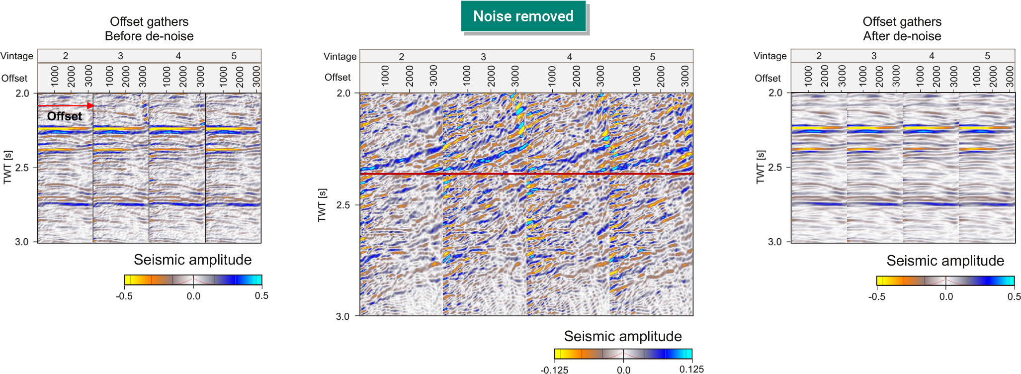
Applying gather conditioning workflows to multidimensional volumes.
The example above shows the effect of applying Radon demultiple on migrated offset gathers from four monitor surveys. Data from all offsets and all vintages are held in one big multidimensional data volume. Differences (middle image) between any gathers before and after applying the demultiple process are calculated interactively and in memory. Amplitudes are scaled by a factor of four in the difference image to enhance the display of the multiples.
How can the signal-to-noise ratio in 4D seismic differences be improved?
Your Subtitle Goes Here

This really depends on the dataset. You have access to a wide range of processing tools, such as random noise attenuation, global and trace-by-trace matching filters, bulk time shifts and time-varying time shifts, to name a few. All tools can be applied to multidimensional datasets, and applied simultaneously to all vintages.
How can I visualize and measure 4D data quality for multiple monitor surveys and track improvements in data quality through gather conditioning workflows
Your Subtitle Goes Here

You can measure 4D data quality and signal/noise ratio by creating maps of quality metrics. This shows you where in your dataset, at what offset, and for which vintage pairs further data quality improvements may be indicated. A rich toolkit with multiple industry standard metrics can be used to quantify data quality measures for multiple repeat surveys and each source-receiver offset or angle for user defined intervals. This process can generate hundreds of maps, stored in multidimensional map objects. You can interactively scroll through the maps, investigating how 4D data quality changes with offset and vintage pairs.
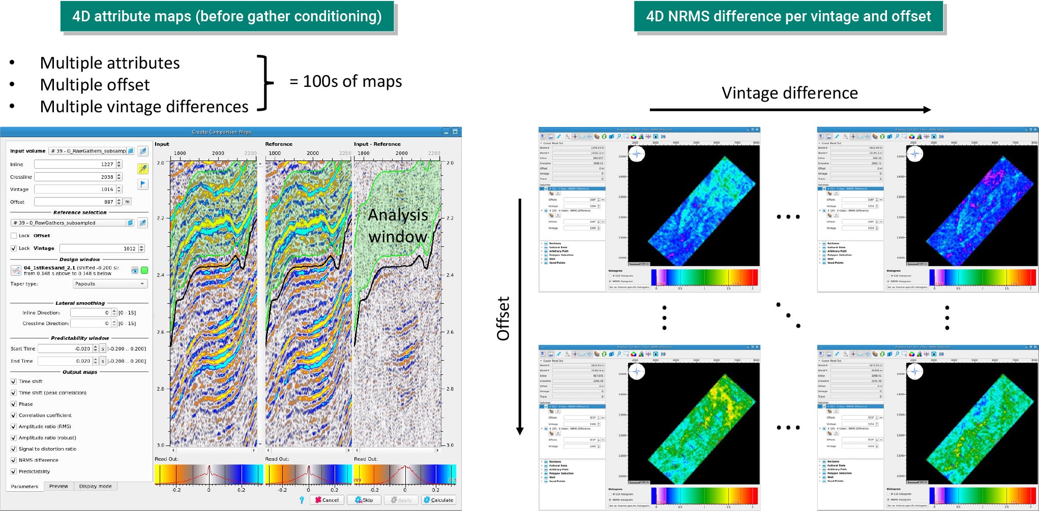
Measuring 4D data quality in raw gathers.
This example shows how multiple attributes are simultaneously extracted for all source-receiver offsets and multiple vintage differences across a 4D dataset. The results are multidimensional map objects, allowing you to interactively scroll through the hundreds of generated maps, and investigate data quality for vintage pairs and offsets.
Is the repeatability of the time-lapse seismic data good enough to confidently detect and quantify 4D seismic differences?
Your Subtitle Goes Here

You can track improvements in 4D data quality through the processing workflow by creating quality control maps after each processing step, and you can assess the improvement in data quality after each step. By comparing the ambient 4D noise level (from nonproducing areas of the subsurface) with the strength of the 4D signal (from synthetic seismic or 4D signals across producing intervals), you can track the improvement of the 4D signal/noise ratio to assess detectability and measurability of 4D signals.
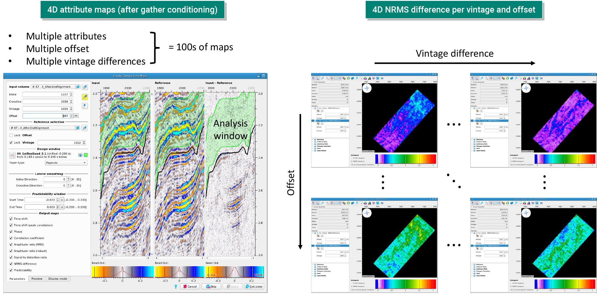
Measuring 4D data quality in conditioned gathers
Comparing QC maps before (see previous question’s picture) and after gather conditioning (the picture above) shows significant improvement in the 4D data quality for all vintage pairs and offsets.
Can I remove production induced time-lapse time shifts?
Your Subtitle Goes Here

Of course. These time shifts can be simultaneously estimated for all vintages in a multivintage dataset, as well as across angles or offsets within a vintage. This markedly simplifies the processing of multivintage and prestack datasets. Algorithm parameters can be interactively tested, and the resulting time shift and time strain output volumes interactively QC’d.
Production induced time-lapse time shifts vary from trace to trace, and along each trace. These time shifts can be measured and removed using a number of different algorithms. In datasets with production induced time-lapse time shifts, this process will increase repeatability between base and monitor surveys. In this respect the process of measuring and removing time-lapse time shifts is similar to any of the other survey matching tools discussed above, with the common goal of improving repeatability, reducing 4D noise and improving 4D signal fidelity.
On the other hand, unlike the other processing steps, the time shifts and time strains measured here can be linked back to production processes. They are therefore also a time-lapse seismic signal, and they are more than yet another step to improve the time-lapse signal. In this respect they are different from global or trace-by-trace matching algorithms between baseline and monitor surveys.
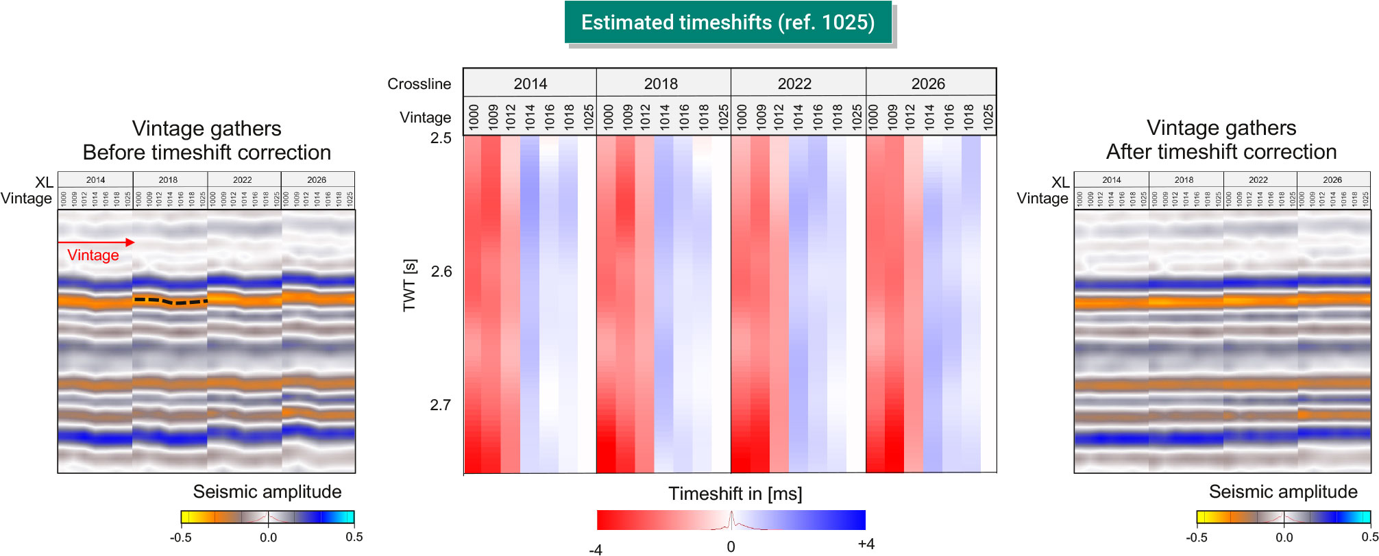
Multivintage time-lapse timeshift estimation and correction. In one process, all vintages and all angle-band stacks.
In the example above, input and output data are displayed as vintage pseudo-gathers, with survey date increasing from left to right within each subpanel. On the input data (left), subtle time shifts are observed on all strong reflections across vintages. These timeshifts have been removed on the resulting output gathers (right). Measured time shifts with respect to the newest survey are shown (center display), and all vintages have been aligned to the newest survey in the aligned gathers. Data courtesy of Equinor.
Reservoir Interpreter and Quantitative Interpreter (QI) specialist
How does Sharp Reflections software handle multiple vintages of prestack seismic amplitude data and attribute data?
Your Subtitle Goes Here

Like all data in Sharp Reflections software, multiple vintages of seismic data can make use of a multidimensional data model, whereby seismic traces are stored in 5D trace “ensembles.” In 4D seismic, the five dimensions are (i) inline, (ii) crossline, (iii) time or depth, (iv) source-receiver offset or incidence angle, and (v) seismic vintage. Note that you do not have to work with prestack data, and the data model works just as well with multiple vintages of stacked data.
Traditional pairwise computations in time-lapse seismic between two surveys have been replaced with an approach that permits simultaneous handling, processing and analysis of all vintages and creation of attributes per vintage.
This simplifies data management, as only one multidimensional data volume is required to store each set of results instead of multiple volumes. Maybe even more importantly, time-lapse differences are computed on-the-fly and in real-time. This avoids pre-calculating and storing the multitude of possible combinations of time-lapse differences.
Can you give some examples of how this assists analysis of multivintage 4D seismic attribute data?
Your Subtitle Goes Here

Sure. Let’s take the example of map-based analysis of 4D amplitude differences between baseline and monitoring surveys. This can generate a large number of maps for each reservoir interval.
Now imagine creating difference maps for various attributes (such as intercept and gradient, inversion attributes, extended elastic impedance, frequency bands, etc.), and attributes for a number of horizons or intervals (required in the analysis of stacked pay). The number of maps an interpreter may want to investigate easily goes into the hundreds or thousands. In traditional approaches, the creativity of an interpreter can become limited by the inability to calculate, keep track of and manage these attribute maps in a data tree.
Our approach automates the generation of instantaneous and interval attributes from all vintages for each producing interval, with differences between any pair of survey vintages calculated interactively. Overall changes are easy to detect on the attribute maps, and production processes such as water injection, water flood, changes in gas-oil ratio, and gas exsolution can be detected using appropriate attribute maps.
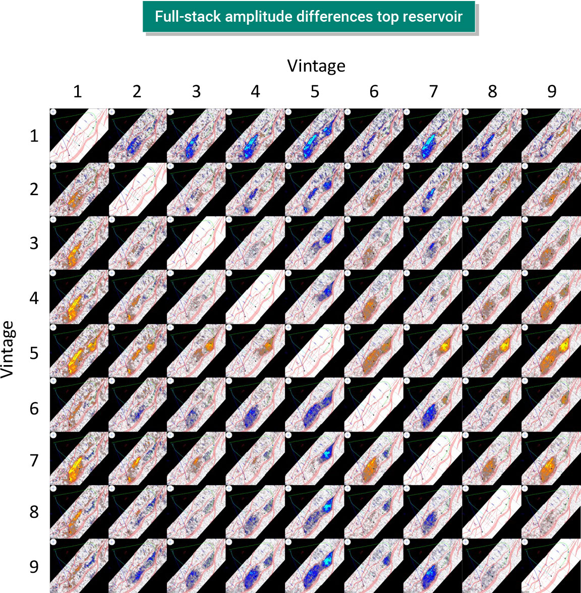
Full-stack amplitude differences, calculated consistently as newer vintage amplitude minus older vintage amplitude, at the top reservoir horizon.
In the example shown here, nine vintages generate 81 possible difference pairs, with 36 unique nondiagonal combinations (and zero differences along the matrix diagonal). Blue colors indicate a hardening response and orange colors indicates a softening response. Data courtesy of Equinor.
Can I create multivintage inversion products?
Your Subtitle Goes Here

Yes. One way to achieve this is to invert each vintage gather to acoustic impedance (AI) and Vp/Vs ratio using a simple Bayesian prestack relative inversion. This inversion is derived entirely from the seismic data, using a simple prior model of a constant background model and allowing a wide range of perturbations in elastic properties. This avoids the creation of a complex model of lithology and fluid classes (LFCs).
A statistical wavelet can also be generated directly from the seismic data. We have had good experiences using this simple approach, and believe that this is a case of “less is more.” Even in situations where the inverted AI and Vp/Vs values do not match the dynamic range of log measurements at well locations, the relative differences between surveys have proven to be remarkably robust, and mapped differences are useful in mapping pressure fronts and water sweep in the reservoir.
The simplified approach removes some of the complexities that made AVA inversions a specialist’s tool and it opens the door for inversions to be used by a generalist interpreter. Coupled with the high-performance computing framework, AVA inversion products can now be created and interpreted in a time frame of minutes.
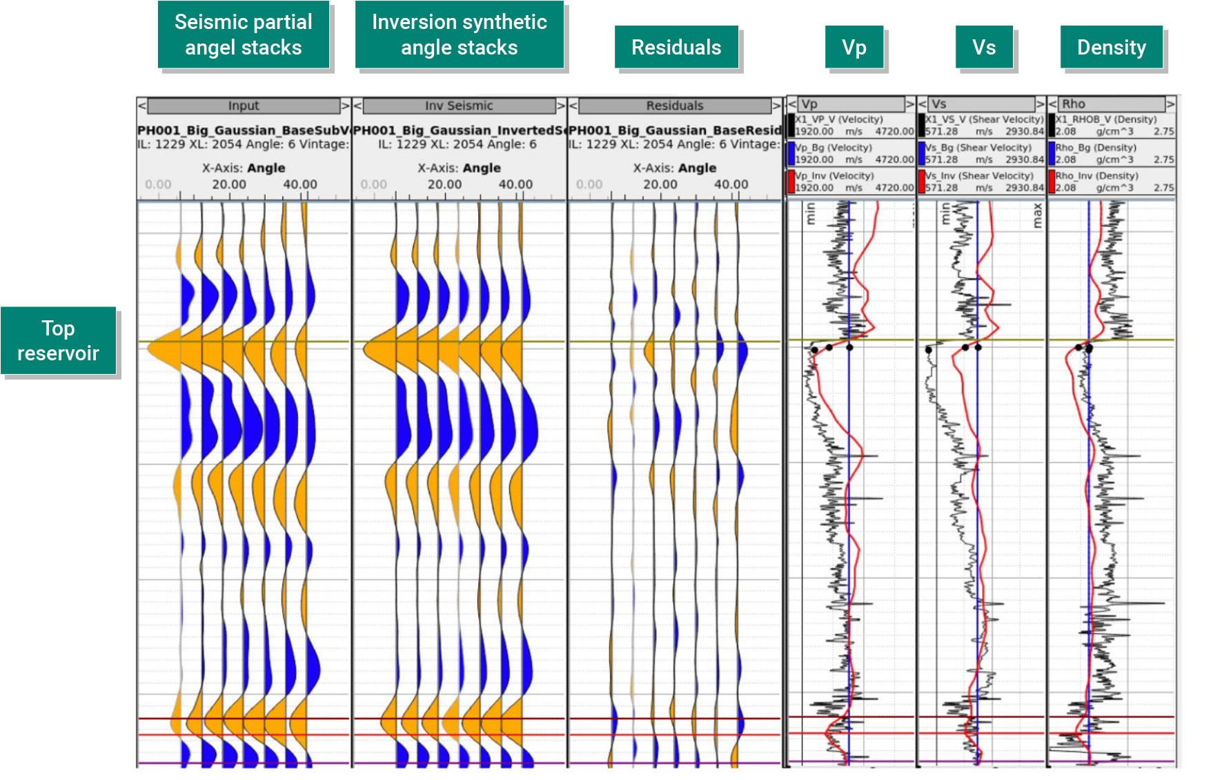
Results from prestack relative inversion at a single blind well location.
The figure shows that inverted Vp, Vs and density curves closely mimic the main trends observed in the well logs, although the dynamic range of the inverted data is somewhat reduced. This mismatch may be reduced by adjusting the scaling of the wavelet used for inversion, without affecting relative differences between surveys.
Which time-lapse seismic attributes are most useful for detecting and quantifying reservoir fluid and pressure changes, as well as reservoir geomechanical changes?
Your Subtitle Goes Here

To help separate pressure and saturation effects, you can use detailed cross-plot analysis. Here we show an example to map the change in AI and VpVs ratio (from the relative prestack inversion shown above) as a function of calendar time, and relate these to pressure and saturation changes measured downhole in wells or estimated from 3D reservoir simulations. Our inversion-based approach simplifies the analysis, since elastic property changes to pressure, fluid fill, and water and oil saturation can be derived from rock physics models.
Alternative means of achieving the same goal do, of course, exist. For example, cross-plotting of differences in multivintage EEI (extended elastic impedance) achieves similar results. This can be done by extracting intercept and gradient in multivintage volumes, combining these into multivintage elastic impedance volumes at pressure and saturation angles, and extracting layer or horizon attributes from these.
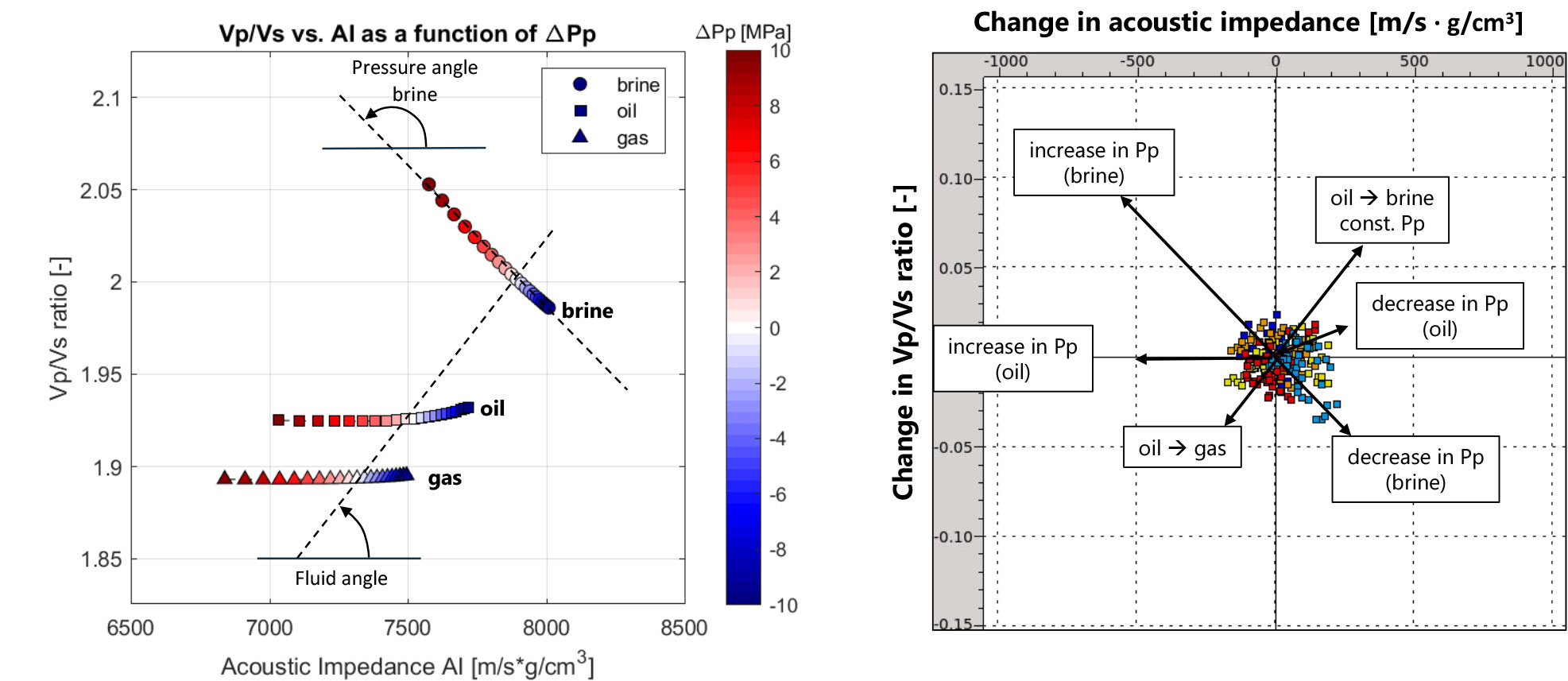
Predicted AI and Vp/Vs due to changes in pressure and saturation, from rock physics model (left). Cross plot of differences in AI and Vp/Vs in nonproducing part of the field, with arrows showing expected directional movement due to changes in pressure and fluid phase (right).
In this figure, actual inverted seismic data points (colored by vintage pairs) are shown in an area where no production effects are expected. The scatter in the plot gives an indication of 4D noise levels in the inversion products.
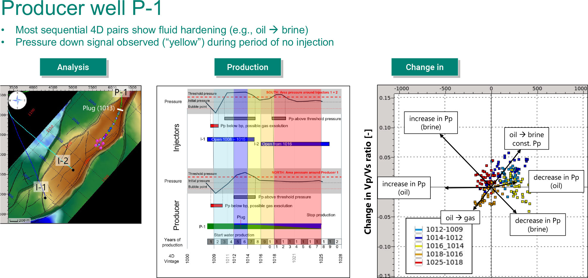
The rock physics model relates ΔAI and ΔVp/Vs to changes in pore pressure and Swater, Soil, Sgas, which can be used to analyze temporal changes in specific map locations with the aid of regionally restricted cross-plots.
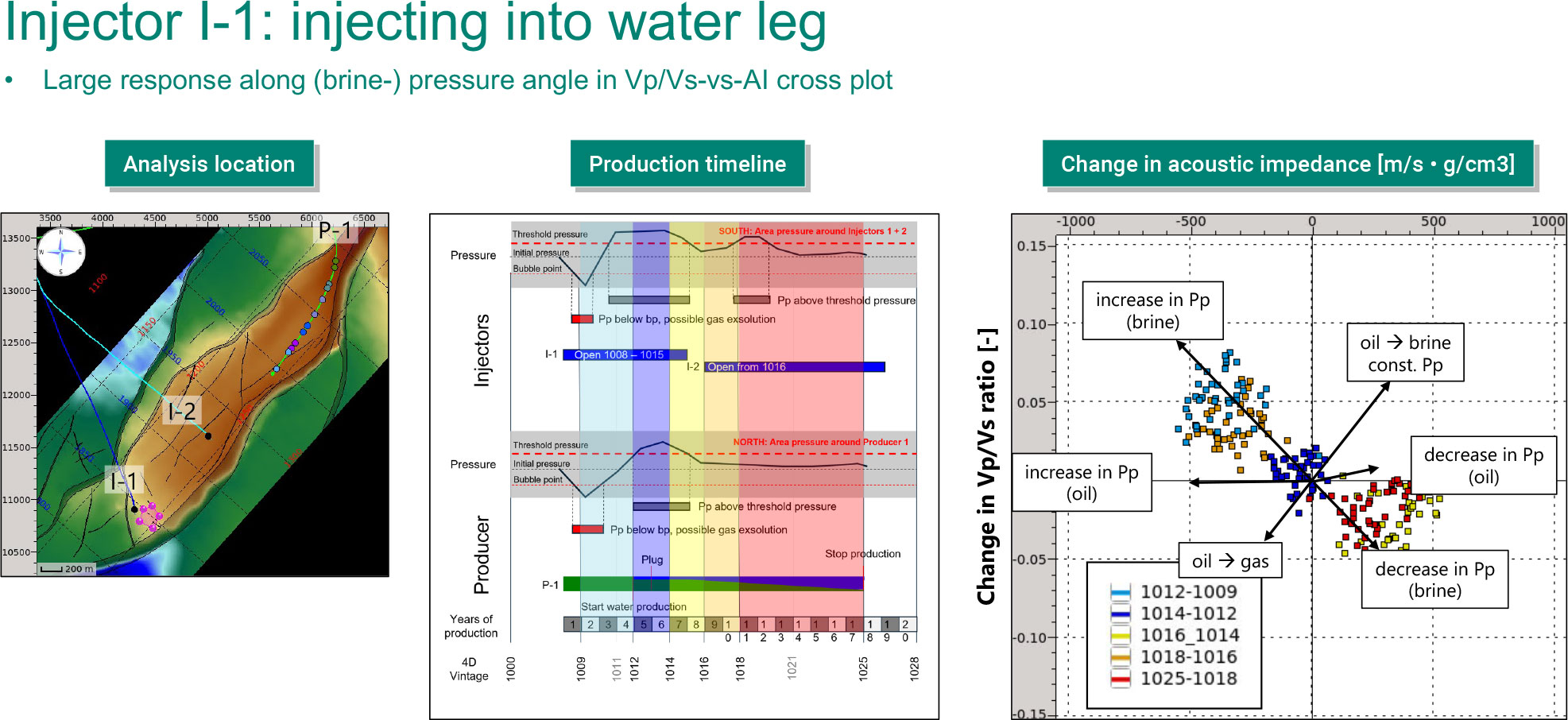
Differences in inverted relative ΔAI and ΔVp/Vs for successive vintage pairs at two different map locations in a producing fault block containing the reservoir.
In the figure above, incremental differences are color coded by survey vintage pairs. Near the I-1 injection well location (left), points move along the NW-SE diagonal, as expected for pressure changes in the brine leg. Differences are consistent with known pressure trends in the field. Near the toe of the P-1 production well (right), difference pairs move in directions suggesting combined pressure and saturation effects, with clear indications of hardening due to water replacing oil.
Key technical capabilities
Core functionality for analysis and interpretation
Vintage axis in 5D data model facilitates efficient time-lapse data processing, analysis, visualization and data management
Multivintage tools and workflows allow concurrent gather conditioning, cross-equalization, analysis and interpretation of multivintage seismic data
Automated comparison tools facilitate comparisons between monitor surveys and a user-defined baseline survey
Horizon decks create a collection of interpreted horizons and infill ghost horizons, enabling simultaneous extraction and storage of horizon and layer attributes for each horizon and layer in the deck
Efficient viewers and spin-box controls support browsing along all five data dimensions of the vintage data, and show on-the-fly time-lapse differences
Amplitude variation with angle (AVA) analysis and 4D inversion analyze and evaluate the time-lapse amplitude-vs-angle signal for reservoir pressure and saturation changes
Map-based time-lapse attribute analysis creates and enables examination of horizon and interval based time-lapse attributes, using map displays and linked cross plots
Dedicated tools for time-lapse processing, modeling, inversion and analysis
4D data quality metrics measure and report repeatability between vintages, also after gather conditioning and cross-equalization of multivintage data
Time-lapse cross-equalization corrects frequency, amplitude, phase and arrival time differences between vintages using trace-by-trace or global matching of time-lapse datasets
Time-lapse time shift estimation and correction tools to measure, correct and analyze production induced time-lapse time shifts and time strains
What-if scenario modeling of the expected time-lapse seismic signal from blocky models or well-log scenarios of fluid and pressure substituted subsurface models
To learn from our experts how to do all this in a real project, sign up for this course:
Dive into the details
Sharp Reflections software equips users to explore complex, multidimensional data volumes interactively using five toolkits. Users move smoothly across the entire spectrum of workflows, from data processing and conditioning through to 4D time-lapse interpretation, all on one platform.

Prestack Data Enhancement
Optimize the reliability of your seismic data.

Quantitative Amplitude Interpretation
Sharpen reservoir insight with multistep QAI analysis. Dive deeper

Inversion
Improve reservoir delineation and net-pay estimation.

Azimuthal
Improve illumination and understanding of complex geological structures.
All the data for the best decisions
Sharp Reflections is the industry’s only software platform built on a powerful compute and display engine designed specifically for HPC, for use on your premises or in the cloud.
Our integrated platform enables you to start analyzing and interpreting seismic data as soon as processing begins. All information contained in the data is mined as you reduce uncertainty and fine tune your reservoir characterization to help achieve trustable exploration, drilling and production decisions.

Connect with us to start your journey to unlock your seismic datasets
Tell us a bit about yourself, and we’ll get back to you.

